Test-time compute in LLM reasoning: what does it actually measure?
An LLM can spend more inference compute by sampling, verifying or adapting its reasoning budget. The useful measure is not answer length, but the trade-off between quality, cost, latency and reliability on representative tasks.
Test-time compute is the extra computation spent while a model produces an answer. Instead of limiting every question to one generation, a system can explore several paths, verify a solution, search a decision tree or adapt its budget to difficulty. This family of methods helps explain recent progress in reasoning models, but it is often reduced to the inaccurate instruction to let the model think longer.
The short answer
Test-time compute measures a compute-allocation policy, not an abstract capability called reasoning. To evaluate it, hold the model, prompt, tools and task set constant, then plot quality against tokens, FLOPs, cost and latency. Compare at least a single generation, multiple samples with aggregation, verifier-based selection and an adaptive stopping rule. Segment results by difficulty and check final answers with an independent oracle whenever possible.
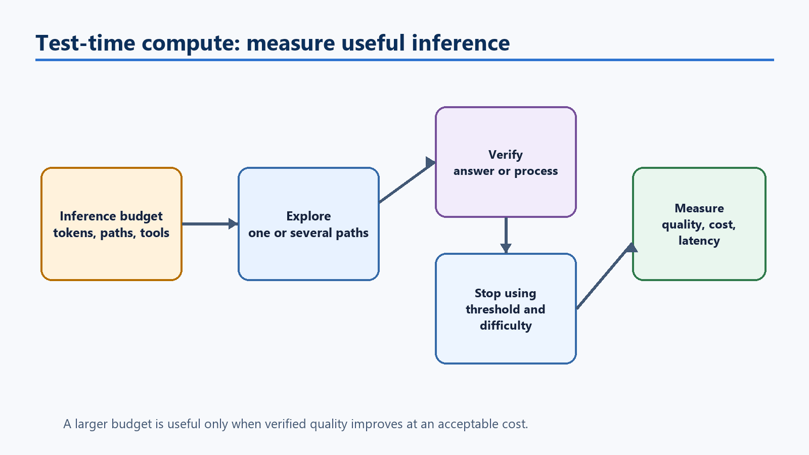
Nexxom diagram. The same model can receive different inference budgets. Evaluation must connect that budget to verifiable quality and operational cost.
What exactly is being measured?
Training compute changes learned parameters before deployment. Inference-time compute does not change the weights: it spends more resources on a particular request. It can mean more reasoning tokens, several parallel trajectories, sequential search guided by a score or calls to tools.
OpenAI explains in its o1 presentation that performance improves with time spent thinking and with training compute. The o1 system card also states that results depend on the checkpoint, system and evaluation protocol. The useful conclusion for an engineering team is not that a high budget is always better. The budget is an experimental variable that must be documented.
DeepSeek-R1 describes another part of the picture. The DeepSeek-R1 paper studies reinforcement learning for reasoning behaviours and releases distilled models. Training compute and test-time compute are not interchangeable. A model may be trained to use an inference budget, but that budget still has to be measured on the intended tasks.
Which strategies should be compared?
A single generation
Greedy decoding or one sampled answer is the baseline. It is fast and easy to log. Without it, a result reported after ten trajectories does not show how much of the gain came from the extra computation.
Multiple trajectories and aggregation
Best-of-N generates N answers and chooses one with a score or a majority. Self-consistency aggregates answers that converge on the same result. This strategy uses parallelism, but it can repeat the same error and raises cost roughly with N. The protocol should publish N, temperature, seed and selection rule.
Outcome or process verification
A verifier can score a final answer, an intermediate step or a computable invariant. Outcome verification fits tasks with an oracle, such as a unit test or a numerical equality. A process verifier can catch an invalid step earlier, but it introduces a second model whose calibration must be tested. A verifier score is not proof: measure false positives and false negatives.
Sequential search and adaptive budgets
Tree search or a stopping rule can allocate more compute to difficult questions and stop easy ones earlier. The Snell et al. study reports, on its tasks and protocol, that optimal inference-compute allocation can outperform simply increasing model size. That is an experimental result, not a universal constant. The s1 paper also studies inference-time scaling with a controlled token budget.
More tokens do not automatically mean better reasoning
A long answer can contain detours, repetitions or an error copied several times. Token count measures spend, not validity. A short answer can be correct when the task is easy. Separate four variables:
| Variable | Question measured | Example logging |
|---|---|---|
| Quality | Does the answer meet an external criterion? | exact match, passed tests, blind human score |
| Compute | How many resources were spent? | generated tokens, calls, estimated FLOPs |
| Latency | How long does the user wait? | p50, p95, tool time included |
| Reliability | Does the result remain stable? | seed variance, abstention rate |
Report these dimensions together. An accuracy-only curve hides the price of the gain. A token-only curve can penalize an efficient verifier. When FLOPs are unavailable, state the chosen proxy precisely and do not present it as a hardware measurement.
A minimal experimental protocol
1. Define the task and oracle
Start with the decisions the system must make: answer a regulatory question, produce a patch that passes tests, classify an incident or calculate a result. Define an independent oracle, a double-annotated human rubric or an executable test. Keep tasks without a verifiable criterion out of the main table.
2. Freeze comparison factors
Model, version, system prompt, tools, temperature, maximum length, context and truncation rules must remain identical across budgets. If one method receives an extra tool, make it a separate experimental condition. The HELM evaluation guide illustrates why scenarios, metrics and constraints should be documented instead of publishing one score.
3. Stratify difficulty
Separate easy, medium and hard questions with a rule defined before the experiment. An adaptive budget can look excellent on average while spending almost all compute on a few cases. Report quality by band together with mean and p95 budget. If difficulty is estimated by the model, validate the estimate on an annotated sample.
4. Measure the cost-quality curve
Test a grid of budgets, such as 1, 2, 4, 8 and 16 trajectories or increasing token limits. For every point, give a confidence interval, sample count, estimated cost and latency. Find the diminishing-return point: the first budget that no longer improves quality beyond the accepted uncertainty.
5. Control contamination and adaptation
A public benchmark may have appeared in training or evaluation traces. Keep a private, time-split or human-verified generated set. Do not change the prompt after seeing a result without creating a new condition. The Simple test-time scaling paper and the critical analysis It's Not That Simple show why protocol and length constraints can change the interpretation of a gain.
A product decision table
| Observed situation | First strategy to test | Success measure | Risk to monitor |
|---|---|---|---|
| Answer can be checked by a test | Multiple trajectories plus verifier | tests passed per euro | poorly calibrated verifier |
| Short numerical answer | Self-consistency or exact oracle | accuracy and median cost | repeated shared errors |
| Difficulty varies widely | Adaptive budget with stop threshold | quality at fixed mean cost | biased difficulty estimate |
| Long, controllable process | Search guided by invariants | valid steps and final result | intermediate score error |
| Open task without oracle | Short sampling and blind human review | preference, factuality, abstention | judge and variance bias |
What test-time compute actually measures
It measures the effectiveness of a compute policy in a specific context. The policy includes the model, generator, verifier, tools, budget and stopping rule. Two systems with the same token count can have different quality if one explores diverse trajectories while the other repeats the same continuation.
The right comparison unit is therefore a reproducible curve, not a spectacular answer. Keep candidate outputs, verification scores, errors, costs and seeds when confidentiality allows. For an API, add a version identifier and the price applied on the test date. For a local system, record hardware, throughput and the FLOPs estimation method.
Production: a simple rule
Start with the smallest budget that reaches the business quality threshold. Increase compute only if the gain persists on a private set and p95 latency remains compatible with the experience. Add abstention or human escalation when the verifier is uncertain. Re-run the curve after every model, prompt, provider or price change.
This avoids two symmetric mistakes: paying for unnecessary thinking on easy requests and confusing a longer answer with a more reliable answer. Test-time compute is an architecture and evaluation lever. It becomes a product capability only when tied to an oracle, a cost and an operational decision.
A reporting template that survives review
For every run, record the model identifier, deployment date, prompt hash, tool configuration, random seeds, maximum output length and budget policy. Store the candidate answers separately from the selected answer so that a reviewer can inspect whether the verifier discarded a correct path. Report the number of examples removed, the reason for removal and the confidence interval method. If a human judge is used, blind the model name and randomize presentation order. These details make it possible to distinguish a genuine allocation gain from prompt tuning, benchmark leakage or a change in the scoring rule.
When the curve is flat, prefer the cheaper point and keep the larger budget as an escalation path. When the curve is unstable, add examples before adding more compute. A stable, slightly lower score can be preferable to a higher average with a large tail of failures. This is especially important for customer-facing workflows where p95 latency and abstention behaviour matter as much as mean accuracy.
Primary sources and further reading
- OpenAI, Learning to reason with LLMs
- OpenAI, o1 System Card
- DeepSeek-AI, DeepSeek-R1
- Snell et al., Scaling LLM Test-Time Compute Optimally
- Muennighoff et al., s1: Simple test-time scaling
- Liu et al., It's Not That Simple
- Stanford CRFM, HELM
- HELM GitHub, scenarios and metrics